Just Enough Statistics
The average that lies
Ten people work in a small office. Nine of them earn ₹30,000 a month. The tenth is the owner, who takes home ₹10,00,000 a month. What is the average salary in this office?
Add them up and divide by ten: ₹1,27,000. Now picture a job ad that says "our average salary is ₹1,27,000". It is mathematically true. And it is completely misleading, because nine out of ten people earn less than a quarter of that.
Statistics is mostly about describing data honestly, with a few numbers that do not lie like that one. You do not need a statistics degree for machine learning. But you do need about five ideas, and you will use every one of them in the chapters ahead. This lesson covers exactly those five.
Idea 1: mean, median and mode
There are three common ways to describe "the middle" of your data:
Key Points
- Mean: add everything up and divide by how many there are. What people usually call "the average".
- Median: sort the values and take the one in the middle. Half the values are below it, half are above.
- Mode: the value that appears most often.
Back to the office. Sort the ten salaries and the middle is ₹30,000. That is the median, and it describes a typical person in the office far better than the mean of ₹1,27,000.
1import numpy as np
2
3salaries = np.array([30000] * 9 + [1000000])
4print("Mean:  ", salaries.mean())
5print("Median:", np.median(salaries))Mean: 127000.0 Median: 30000.0
Why the huge gap? The mean uses every value, so one extreme value drags it a long way. The median only cares about the middle position, so the owner's salary barely affects it.
Tip:A simple rule: for salaries, prices, rents and anything else where a few values can be huge, report the median. When there are no extreme values, the mean and median are close, and the mean is fine.
The mode is most useful for categories, where mean and median make no sense. What is the average area in Pune? A meaningless question. But the most common area is a fair one. In our flats data, Baner, Kothrud and Wakad tie with 4 flats each, which shows that data can have more than one mode.
Idea 2: spread
Here are the marks of five students in two different classes:
Key Points
- Class A: 68, 70, 70, 72, 70
- Class B: 40, 55, 70, 85, 100
Both classes have a mean of exactly 70. If you only knew the average, they would look identical. But they are completely different. In class A everyone is at about the same level. Class B has someone struggling and someone topping. The average hides this. What it hides is called spread.
The simplest measure of spread is the range: highest minus lowest. Class A has a range of 4, class B a range of 60. Easy, but fragile. A single extreme value changes it completely.
The measure everyone uses is the standard deviation (often shortened to std). In plain words, it is the typical distance of a value from the mean. Here is how it is worked out for class B, step by step:
Key Points
- Find the mean: 70.
- Find how far each mark is from it: -30, -15, 0, 15, 30.
- Square each distance, so negatives do not cancel out positives: 900, 225, 0, 225, 900.
- Average those squares: 2,250 ÷ 5 = 450.
- Take the square root, to get back to the original units: √450 ≈ 21.2.
1class_a = np.array([68, 70, 70, 72, 70])
2class_b = np.array([40, 55, 70, 85, 100])
3print("Class A:", class_a.mean(), "give or take", class_a.std().round(1))
4print("Class B:", class_b.mean(), "give or take", class_b.std().round(1))Class A: 70.0 give or take 1.3 Class B: 70.0 give or take 21.2
Now the two classes look as different as they really are. "70, give or take 1.3" versus "70, give or take 21.2". You do not need to calculate this by hand ever again. Just remember what it means: small std, values huddle close to the mean. Big std, values are spread far and wide.
Percentiles and the quick summary
One more idea about spread that you will see constantly. The 25th percentile is the value that 25% of the data falls below. The 50th percentile is the median. The 75th percentile is the value 75% falls below. Together they tell you where the middle half of your data lives.
pandas gives you all of this in one line with describe(). Here it is for the Pune rents:
1import pandas as pd
2
3df = pd.read_csv("https://cod-e.vercel.app/data/pune-flats.csv")
4df["rent"].describe().round()count 21.0 mean 26690.0 std 10249.0 min 13500.0 25% 20000.0 50% 26500.0 75% 30000.0 max 54000.0 Name: rent, dtype: float64
Read it like a story. 21 flats. The typical rent is around ₹26,500 (the median), give or take about ₹10,000. The cheapest is ₹13,500 and the most expensive ₹54,000. And the middle half of all flats rent for between ₹20,000 and ₹30,000.
Tip:Run describe() on every new dataset, right after head(). It takes one second and often catches problems straight away, like a minimum rent of 0 or a maximum that is clearly a typo.
Idea 3: the shape of the data
In the Matplotlib lesson, the histogram showed you the shape of the rents. That shape is called the distribution, and two shapes come up again and again:
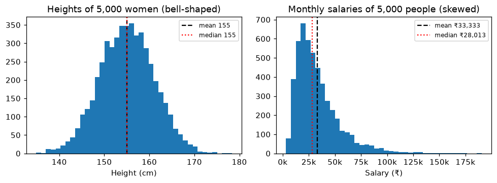
On the left is the bell shape, also called the normal distribution. Most values bunch around the middle and thin out evenly on both sides. Heights, exam marks in big exams and small measurement errors often look like this. The mean and median sit right on top of each other.
A handy fact about bell shapes: about 68% of values fall within one standard deviation of the mean, and about 95% within two. If women's heights average 155 cm with a std of 6 cm, then roughly 95% of women are between 143 and 167 cm.
On the right is a skewed distribution. Most people earn a modest amount, and a long tail of high earners stretches off to the right. Salaries, prices, rents, delivery times and website visits usually look like this. The tail drags the mean towards it, so the mean ends up above the median.
Tip:A quick clue without drawing anything: if the mean is much bigger than the median, the data probably has a long tail on the right. That is exactly what happened with the office salaries.
Idea 4: outliers
An outlier is a value that sits far away from all the others. The owner's salary is one. The ₹54,000 flat in Viman Nagar is one.
The important question is not "is it an outlier?" but "is it real?":
Key Points
- Some are mistakes. Meera's 4,120-thali day in lesson 1.5 was really 412, with an extra zero typed. Mistakes should be fixed.
- Some are real and important. A large, furnished 3BHK in an expensive area really does cost ₹54,000. Deleting it would teach the model that such flats do not exist.
So never delete outliers automatically. Look at them and ask what they are. Chapter 3 covers how to find and handle them properly.
Idea 5: correlation
In lesson 2.5, the scatter plot showed that bigger flats tend to cost more. Correlation turns that "tend to" into a single number between -1 and 1:
Key Points
- Close to 1: when one goes up, the other goes up too, very reliably.
- Close to 0: no clear straight-line relationship.
- Close to -1: when one goes up, the other reliably goes down. Like a phone's age and its resale price.
1df[["size_sqft", "floor", "rent"]].corr().round(2)size_sqft floor rent size_sqft 1.00 0.12 0.88 floor 0.12 1.00 0.02 rent 0.88 0.02 1.00
Find the rent column and read down it. Size and rent: 0.88, a strong relationship. Floor and rent: 0.02, almost nothing. (The 1.00s are each column compared with itself, which always gives exactly 1.) Here is what those two numbers look like:
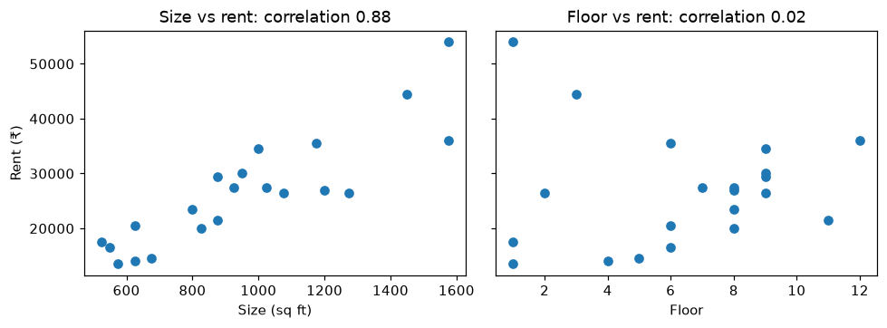
This is why correlation matters for ML. It is a quick first check of which features are likely to be useful. Size looks very useful for predicting rent. Floor, in this data, does not.
Correlation is not causation
This is one of the most important ideas in all of data work, so it gets its own section.
In a city, umbrella sales and traffic jams are strongly correlated. On days when lots of umbrellas are sold, the roads are jammed. Does buying umbrellas cause traffic jams? Of course not. Rain causes both. Rain is the hidden third thing driving the two numbers together.
Correlation only tells you that two things move together. It never tells you why. A model will happily use a correlated feature to make predictions, and that is fine. But when someone says "X causes Y" based on a correlation alone, be sceptical.
Why ML needs all five
Key Points
- Mean and median: filling in missing values is often done with one of these. (Chapter 3)
- Standard deviation: feature scaling uses it to put features on a similar scale. (Chapter 3)
- Distribution: tells you whether to trust the mean, and shapes how you measure a model's errors. (Chapters 3 and 4)
- Outliers: can badly throw off some models if they are mistakes. (Chapter 3)
- Correlation: a quick first check for useful features. (Chapter 3)
Where people get confused
Key Points
- "The average is always the best summary." For skewed data like salaries and rents, the median is usually more honest.
- "A correlation of 0 means the two things are unrelated." It means there is no straight-line relationship. They could still be related in a curved way.
- "NumPy and pandas gave me different standard deviations for the same numbers!" They use slightly different formulas by default. pandas divides by one less than the count. For class B above, pandas gives 23.7 instead of 21.2. On large datasets the difference becomes tiny.
- "Outliers are errors, so delete them." Some are errors, some are the most important rows you have. Check before deleting.
Quick check
A news report says the "average house price" in a city is ₹2 crore, but most people you know live in far cheaper homes. What might be going on?
House prices are skewed. A few very expensive homes drag the mean far up. The median would probably be much lower and closer to what a typical home costs.
Two delivery apps both average 30 minutes per order. One has a std of 3 minutes, the other 15. Which would you trust for an important lunch?
The one with the std of 3 minutes. It almost always arrives in about 27 to 33 minutes. The other could easily take 45 minutes or more.
Ice cream sales and sunburn cases are strongly correlated. Does ice cream cause sunburn?
No. Hot, sunny weather causes both. Correlation shows that they move together, not that one causes the other.
Recap
Key Points
- Mean, median and mode describe the middle. Use the median when extreme values exist.
- Standard deviation is the typical distance from the mean. Small means huddled, big means spread out.
- describe() gives you count, mean, std, min, percentiles and max in one line. Run it on every new dataset.
- Bell-shaped data is symmetric. Skewed data has a long tail that pulls the mean towards it.
- Correlation, from -1 to 1, measures how reliably two numbers move together. It never proves one causes the other.
That is the end of Chapter 2. You now have the whole toolkit: Python, notebooks, NumPy, pandas, Matplotlib, scikit-learn and the statistics to make sense of what they show you.
Next up, Chapter 3: data. Remember the rent model that could not see area or furnishing? We are going to fix it, starting with a question you have been quietly avoiding. Where does good data come from in the first place?
Theia
Can you explain this concept?
Practise Just Enough Statistics with realistic interview questions. Choose spoken or typed answers, get feedback on your reasoning, then return to the material that needs work.
Sign in to practise this conceptThe session stays focused on this lesson. Your selected interview level sets the bar.